Part 22 - Make a query table
with VBA and add calculated columns
Excel can automatically fill in
and update columns adjacent to a query table result set if the
adjacent rows contain cell formulas based on data returned
from a query. That means if your source database changes and
you refresh the query, when the new record set is returned,
all the adjacent cell formulas will calculate new values for
the corresponding rows in the result set, and the number of
rows in the adjacent columns will adjust automatically.
You can make a query from scratch using VBA. Let's put these
two features to the test.
1. Open a new, blank workbook.
2. In the VB Editor, in a new module type or paste the
following macro:
Sub MakeAQuery()
Dim sqlstring As String
Dim connstring As String
sqlstring = "SELECT Products.ProductName,
Products.UnitsInStock, Products.UnitsOnOrder,
Products.ReorderLevel, Products.Discontinued FROM Products
WHERE (Products.ProductName like '%chestnut%')"
connstring = "ODBC;DSN=ExampleData"
With ActiveSheet.QueryTables.Add(Connection:=connstring,
Destination:=Range("A1"), Sql:=sqlstring)
.BackgroundQuery = False
.HasAutoFormat = True
.Refresh
.FillAdjacentFormulas = True
.UseListObject = True
End With
With ActiveSheet
.ListObjects("Table1").TableStyle =
"TableStyleMedium10"
End With
End Sub
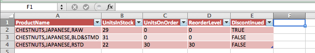
3, Run the macro.
The result set should look like this screen shot:
4. Click into the cell immediately to the right of the field
headers. In this example this cell is F1, as shown in the
screen shot above.
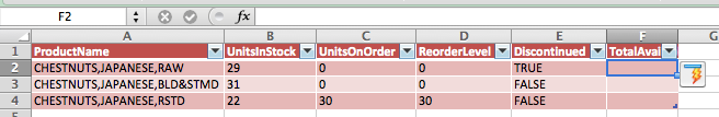
5. Type
a new field name in the selected cell. In this example the new
field name will be TotalAvailable, which will be the sum of UnitsInStock
plus UnitsOnOrder. When you press the Return key on
your keyboard, notice that the formatting fills down, as shown
below.
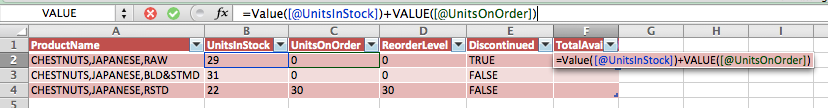
6. Do not click anywhere. You must immediately Press the = key
to begin a cell formula. Your formula starts with =VALUE(
Stop typing. Before continuing, know that all of the records
in the Products table in ExampleData.xls were stored as text,
so our cell formula will treat these values as text.
7. Look at the screen shot below. Build your cell formula
arguments by clicking into cells B2 and C2. Notice that Excel
builds the formula using the column headers rather than cell
references. This is pretty neat. Excel calls this a
"calculated column."
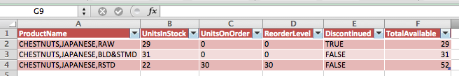
8. Press return and Excel will automatically fill the formula
down. This is very handy if you have thousands or hundreds of
thousands of records to work with.
If data in the data source changes and has been saved, when
you refresh your query the adjacent column's calculated
formulas will recalculate based on the new data and adjust to
the new row count. The formatting of the first record in the
query table will copy down. Sorry, the fancy every other row
formatting won't be retained unless you do more coding. You
can add as many additional columns as you want to your query
table this way. Remember, the name of the table increments
each time you refresh the query.
To obtain a VBA code example of making a calculated column,
click the Record Macro button on the Developer Tab of the
Ribbon between steps 3 and 4 above. Click the Stop Recording
button after step 8. The macro recorder will record the code
you need.
Here's an example of a connection string that was used to
connect to a Microsoft SQl Server
ConnectionString =
"ODBC;DSN=MyDataSourceName;DATABASE=MyDatabaseName;SERVER="192.255.255.255";PORT=5432;UID=MyUserName"